A Novel Numerical Solution Technique for
Linear Boundary Value Problems of
Partial Differential Equations
Abstract:
A numerical method for
the solution of linear partial differential equations (LPDEs) with given
boundary functions is introduced. The significance of this method is in its
directness and simplicity and the versatility of its application to all types
of LPDEs. In three dimensions, for example, with this method the elliptic PDEs
are solved the same way as the hyperbolic and parabolic types. An elliptic LPDE
in two dimensions when discretisized into a rectangular grid of X by Y nodes,
can be considered as a directional derivative functional made of a scalar
product of two vectors in an
2.(X-2)+2.(Y-2) dimensional
space. One of these vectors consists of (n-2) independent functions among the
total and the other is the gradient of the solution at that step with respect
to the components of this vector. Furthermore the 3.(n-2)boundary nodes and the
inhomogeneous part of the LPDE can be stored as one component and so the number
of the vector components reduce to X-2+1=X-1 (or Y-1). With the help of the recursion relation that
is obtained by differencing the LPDE, the gradient vectors can be obtained recursively,
and numerically stored in digital computers that are programmable through any
of the present languages. In other words, through this method we can
effectively self start the solution of any LPDE as would be in an parabolic or
hyperbolic type that are initial value
problems.
Introduction:
The differential
equations arise in scientific and engineering problems naturally as an
expression of the change of the independent variable with respect to the
control variable or variables. In the case of more than one control variable
the problem is called a partial differential equation. Full solutions to the
differential equations are obtained only after the introduction of some
conditions that the desired solution or its derivatives have to satisfy at the
ends. If these end conditions are all at the one and same side, the problem is
a self starter and properly called an initial value problem. For these types of
problems both numerical and, if available, analytical solutions are found
straightaway. The analytical solution, if available, is of course the first
choice. However if the solution cannot be made expressible in terms of any
known analytical functions, the only resort is the numerical approach.
The well known
boundary value problems in physical and engineering applications are: Laplace's
(or similarly Poisson's (an elliptic type), for example, Uxx+Uyy+Uzz
= 0 or C(x,y,z), for the unknown function U(x,y,z,t), where subscripts
denote partial differentiation with respect to the denoted varible as many
times as the repetition) equation; wave equation (for example, Uxx+Uyy+Uzz
= -Utt, an hyperbolic type); diffusion equation (or heat
equation, for example, Uxx+Uyy+Uzz = Ut,
an parabolic type) [1, James]. If we knew the values of the solution U at all
interior points of the solution domain, we would easily propagate them along
the time axis as indicated by the right hand side of the parabolic and
hyperbolic types. But the left hand sides of the above themselves are elliptic LPDEs in terms of x,y, and z. Thus the real challenge is in
computing U(x,y,z,,t0) for the space part only at the initial time t0 in such a
way that U(x,y,z,t0) obeys the spatial boundary functions given with the
problem.
The traditional way of
numerically solving elliptic PDEs is by discretization and Gauss-Seidel
elimination method, for all the (X-2)x(Y-2) unknown nodes. For hyperbolic and
parabolic types solution is obtained with less trouble and a good number of
techniques including method of characteristics are reviewed in Aktas et. al.
[3].
In this paper, we are
to show how the solution to an elliptic LPDE can be obtained with matrices
smaller than those of in the literature. Though the method is general for any
order and for any number of independent variables in LPDE and for any shape of
the solution domain, for sake of
simplicity, we will restrict
ourselves to the solutions of Uxx + Uyy = 0 (elliptic) in a square domain, and we
will show that the solution to the elliptic type can be converted to the
parabolic or hyperbolic types, which are initial value problems where the given
boundary function at one end at time t0 just self propagates to other
times. If we choose (X-1) and (Y-1)
integration steps along x and y axes respectively (which means we are
discretisizing our boundary function along x at X number of points and the
other boundary function along y at Y number of points) we see that U needs to
be calculated at (X-2).(Y-2) nodes.
Among the boundary values at [2.(X-2)+2.(Y-2)+4] nodes only [2.(X-2)+2.(Y-2)]
are needed for the solution, i.e., the ones at the four outside corners are not
needed at all. The traditional way of
attacking this problem is to construct an array of made of
all the U’s at (X-2).(Y-2) nodes which in turn leads to a matrix of (X-2).(Y-2) by (X-2).(Y-2) elements. For any
method of solution, whether it is Gauss-Seidel elimination or triangulation or
matrix inversion, this big a matrix would not be used if we had been given one
of the boundary functions, say the one along the x-axis at the second step of the discretization as would be in an
initial value problem (Fig. 1).
The crucial question
is that can we convert this into that initial type? If we did that, the number of unknowns would be (Y-2). The
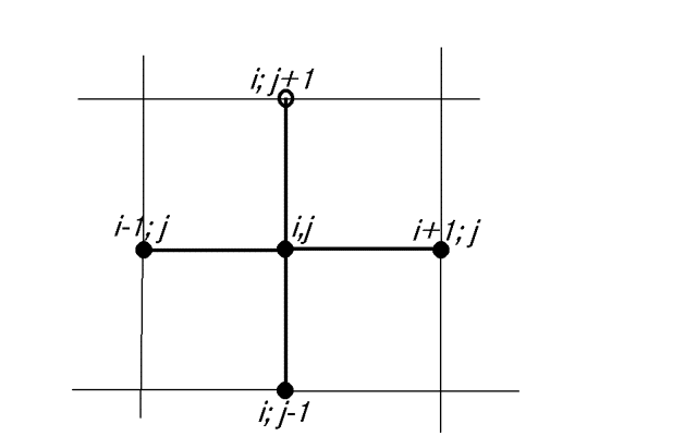
discretization of the LPDE Uxx + Uyy =0 schematically
shows that the nodal value at the top tip of the cross can be expressed as the
combination of the nodal values of the remaining tips and the center, as in
U(i,j+1) = -U(i,j-1)
-U(i-1,j) -U(i+1,j) +U(i,j)/4
for C(x,y,z)=0 (see Fig. 1).
For C(x,y,z) not equal
to zero we need to add C(i,j,k) term to the right hand side. If this is to be
iterated all over the solution domain, practically at the top of the domain we
would get the top y-boundary values. The (X-2).(Y-2) intermediate nodal values
are then expressible in terms of the bottom and top 2.(X-2) nodes and left and
right 2.(Y-2) nodes. However to do this we do not need as large a martix as
indicated in the literature, what we need is a (X-2) by (X-2) or (Y-2) by (Y-2) matrix, depending on our
choice of the march (propagation) direction. Of course, it is more advantageous
to chose the row with smaller number of nodes for the march. In our example,
since the solution domain is square X=Y, and we chose the solution domain is
square X=Y, and we chose the positive y direction as the marching direction.
Our marching row is the row with x=2. The given boundary nodals are
counterclockwise at y=1, x=X, y=Y, and x=1.
Then, if X is the
smaller of X and Y, we can shift the boundary values along negative y
direction down to the second row of the
nodes. From the second row on, the problem is an initial value problem and will
be solved as if it were a parabolic or
hyperbolic LPDE boundary problem.
As in our previous
paper on the numerical solution of linear ordinary differential equations
(LODEs) the nodal value U(i,j+1) will be expressed as the directional
derivative functional in term of the all the boundary nodal values that are
used for the self start and the remaining boundary nodal values that are to be
shifted plus the particular solution. However we can collect all the self start
boundary nodal values (the
inhomogeneous part of the LPDE too) under one variable V and further if
C(x,y,z)=0,
U(i,j+1) =
[U(2,2),U(3,2),...U(X-1,2),V] ·ÑU(i,j+1)
where the left
boundary nodals U(1,2), U(1,3),....,U(1,Y-1), and the right boundary nodals
U(X,2), U(X,3),...,U(X,Y-1) are all together represented in V. The outer corner
nodals U(1,1), U(X,1), U(1,Y), U(X,Y) are not needed for the solution. The “·” represents
the scalar product operator of vectors and “Ñ”
represents the gradient operator with respect to the components of the vector
it is acting on. In analogy to a vibrating mesh of strings case, the corner
nodes can be regarded as the corner pegs at which no strings are attached; whereas
between the other edge nodes horizontal
and vertical strings are stretched, these strings are soldered at the
intermediate nodes (Fig. 1).
Since now, all the
nodal U’s can be expressed in terms of the [...] vector, and the top boundary
specifies the known U(2,Y),U(3,Y),...,U(X-1,Y) values, the unknown set
U(2,2),U(3,2),...U(X-1,2) can be solved in terms of these known values. The
solution requires an (X-2) by (Y-2) matrix solved by inversion or elimination.
Though we demonstrated
the method through a square domain in the example given at the end, we should
stress that the form of the solution domain need not be square or rectangular
and the LPDE need not be given in terms of Cartesian variables for our
technique to be applicable. Generalization to other domains and other
coordinate systems are obvious.
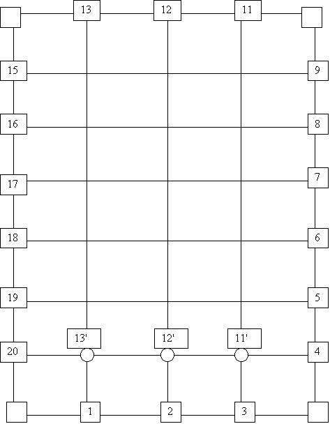
Along the march of the
solution then there should be just enough number of boundary points to be shifted as needed for the march. In any
case one should mark the top boundary points to be shifted noticing the maximum
number of nodes at of the marching rows
(Fig. 2). In higher dimensions of n greater than two, the marching row is a
hypersurface of ‘n-1’ dimensions. One can choose nonsquare or non rectangular grids
by interpolating/extrapolating (or Taylor series expanding) to account for the
grid shape changes [2,3]. The boundary conditions in form of derivatives can be
handled as usual [2].
In the example below,
even though we used a Gauss-Seidel elimination method, it is not the best way
of finding the solution to ‘X-2’ unknowns through ‘X-2’ linear equations. Aim
of this paper is not to investigate the fastest method of solution on a system
of linear equations. Reader is advised
to employ a faster method for the
solution to linear equation systems.
We used the output of
the example given reference [1], page 609 for the comparison with our
method.
Example Code 1:
c PDE: Vector; Gauss-Seidel; square grid and domain
with
c over
relaxation w=1.8; number of iterations=2586; nb=nx-2 or nb=ny-2.
parameter(nx=10,ny=10,nb=8)
real
U1(nx,ny),B(nx,ny), sum(nx,ny), a(nb,nb), c(nb),
&
x(nb), gs(nb), James(nx,ny), sum2(nx,ny), BC(nb),perr(nx,ny)
integer*4 U(nx,ny,nb)
c data from James page 609 with epsilon=0.001 and
nmax=100:
data
James/
& .00,
.00, .00, .00,
.00, .00, .00,
.00, .00, .00,
&
19.06,18.43,17.20,15.95,14.92,14.18,13.70,13.42,13.28,13.24,
&
39.40,37.45,34.42,31.67,29.56,28.11,27.20,26.70,26.47,26.41,
&
63.63,57.56,51.37,46.74,43.56,41.50,40.29,39.69,39.49,39.46,
&100.00,77.78,66.77,60.37,56.42,54.04,52.77,52.30,52.33,52.46,
&100.00,86.78,77.58,71.54,67.72,65.48,64.46,64.42,65.07,65.73,
&100.00,91.78,85.21,80.51,77.42,75.69,75.16,75.85,77.80,80.33,
&100.00,95.12,90.98,87.86,85.78,84.69,84.66,86.03,89.93,100.0,
&100.00,97.71,95.72,94.18,93.15,92.65,92.74,93.67,95.90,100.0,
&100.0,100.0,100.0,100.0,100.0,100.0,100.0,100.0,100.0,100.00/
data
itemax/9 999/
c initialize:
do 20 j =
1, ny
do 20 i =
1, nx
sum2(i,j)
= 0
20 sum(i,j)
= 0
c define boundaries from James's solution array:
do 25 i =
1, nx
B(i,1) =
James(i,1)
25 B(i,ny)=
James(i,ny)
do 26 j =
1, ny
B(1,j) =
James(1,j)
26 B(nx,j)=
James(nx,j)
c interpolate B(i,j):
do 27 j =
2, ny-1
do 27 i =
2, nx-1
By=B(i,1)+(B(i,ny)-B(i,1))/(ny-1.)*(j-1.)
Bx=B(1,j)+(B(nx,j)-B(1,j))/(nx-1.)*(i-1.)
27
B(i,j)=(By+Bx)/2.
do 3 j = 2, ny-1
do 2 i =
2, nx-1
do 1 k
= 1, nb
U(i,j,k) = 0
U1(i,j) = B(i,j)
if((i-1).eq.k.and.j.eq.2) U(i,2,k) = 1
1
if((i-1).eq.k.and.j.eq.2) BC(k) = 0
2 U1(i,1)
= B(i,1)
U1(1,j) = B(1,j)
3 U1(nx,j)
= B(nx,j)
do 5 j =
2, ny-1, 1
do 5 i =
2, nx-1, 1
do 4 k =
1, nb, 1
4
U(i,j+1,k)=-U(i,j-1,k)-U(i-1,j,k)-U(i+1,j,k)+U(i,j,k)*4
5
U1(i,j+1)=-U1(i,j-1)-U1(i-1,j)-U1(i+1,j)+U1(i,j)*4
c Gauss-Seidel:
do 7 i = 1, nb
do
6 k = 1, nb
6 a(i,k) =
U(i+1,ny,k)
c(i)=U1(i+1,ny)-B(i+1,ny)
7
x(i)=BC(i)
w=1.8
dif=0.1
iter=0
22
iter=iter+1
if(iter.ge.itemax)goto 11
do 9 i =
1, nb
gs(i) =
c(i)
do 8 k
= 1, nb
8 gs(i)=
gs(i) + a(i,k)*x(k)
9
x(i)=(-(gs(i)-a(i,i)*x(i))/a(i,i))*(w)+(1-w)*x(i)
if(abs(gs(1)).ge.dif.or.abs(gs(2)).ge.dif.or.
& abs(gs(3)).ge.dif.or.abs(gs(4)).ge.dif.or.
& abs(gs(5)).ge.dif.or.abs(gs(6)).ge.dif.or.
&
abs(gs(7)).ge.dif.or.abs(gs(8)).ge.dif)goto 22
11 write(*,12)(x(i),i=1,nb)
12
format(1x,'x: ', 8(f5.3,1x))
write(*,16)iter
16
format(1x,'iterations=',i8)
write(*,17)(gs(i),i=1,nb)
17
format(1x,'gs :',8(e8.1,1x))
c Back substitude x(k)'s:
do 14 j =
2, ny, 1
do 14 i =
2, nx-1, 1
sum2(i,j)=0
do 13 k
= 1, nb, 1
13
sum2(i,j)=sum2(i,j)+x(k)*U(i,j,k)
sum2(i,j)=sum2(i,j)+U1(i,j)
14
perr(i,j)=(sum2(i,j)-James(i,j))/James(i,j)*100
write(*,29)
29
format(1x,'
Percent errors')
do 28
j=2,nb
28
write(*,15)(perr(i,j),i=2,nx-1)
15
format(1x,8(f5.1,1x))
stop
end
The output:
x: 3.667 2.763
1.835 1.134 .717 .557
.599 .784
iterations= 2586
gs : .5E-01
.9E-01 .7E-01 -.3E-02
-.7E-01 -.1E+00 -.1E+00
-.4E-01
Percent errors
.0
.0 .0 .0
.0 .0 .0
.0
.0
.0 .0 .0
.0 .0 .0
.0
.0
.0 .0 .0
.0 .0 .0
.0
.0
.0 .0 .0
.0 .0 .0
.0
.0 .0
.0 .0 .0
.0 .0 .0
.0
.0 .0 .0
.0 .0 .0
.0
.0
.0 .0 .0
.0 .0 .0
.0
A question ‘Can it be
possible to solve this elliptic PDE with lesser unknowns than ‘X-2’? might be
tempting. The answer is given in the theory of the LPDE’s and it is ‘No’.
Because elliptic PDEs need to know where they are ending at the other boundary
edge, whereas true initial value problems find their proper value at the other
edge by their own. The following code attempts to march to the proper values at
the center from four sides inward. At the each side only two nodal values are
initialized. This is done by using the discrete formula at 45 degrees too, and
at the end of the march that reaches
the other edge, the two nodal values are satisfies. Then the solution marches
towards the center from all four sides while being guided by the edges on the
left and right. This approach totally neglects the fourth edge, and as
expected, at the end the solution is found far off from the true values at the
fourth edge. An elliptic PDE needs full information from all four sides before
any march is started off. We see that, even though the domain is extremely
small, the percent errors are still significant.
Example Code 2:
c An example
for the solution of Uxx+Uyy=0 with BCs
c Forming a rim
from corner to corner four times and then
c marching
towards center for unit step sizes along x and y
c Each rim has
2 unknowns, solved by matching at the
c boundary
nodes accross.
parameter (n=10)
integer*4 u(n,n,2), t(n,n,2)
real*8 v(n,n), r(n,n)
real*8 dx2,
pn2,pn3,pnn1,pnn2,p2n,p3n,pn1n,pn2n
real*8
x,y,f,q,w,z,u22,u23,un1,un2,u2n,u3n,un1x,un2x
real perr(n)
data dx2/0.01d0/
x(ix)=ix/10.d0
y(iy)=iy/10.d0
f(w,z)= dexp(-w*z)
q(w,z)=dx2*(w*w+z*z)*f(w,z)
do 10 j = 1, n
do 10 i = 1, n
v(i,j)=0d0
r(i,j)=0d0
do 10 k = 1, 2
10 u(i,j,k)=0
u(2,2,1)=1
u(2,2,2)=0
u(2,3,1)=0
u(2,3,2)=1
u(2,n-1,1)=1
u(2,n-1,2)=0
u(2,n-2,1)=0
u(2,n-2,2)=1
t(2,2,1)=1
t(2,2,2)=0
t(3,2,1)=0
t(3,2,2)=1
t(n-1,2,1)=1
t(n-1,2,2)=0
t(n-2,2,1)=0
t(n-2,2,2)=1
c define
boundary nodals
do 2 i=1,n
v(i,1) = f(x(i),y(1))
v(i,n) = f(x(i),y(n))
v(1,i) = f(x(1),y(i))
v(n,i) = f(x(n),y(i))
r(i,1) = f(x(i),y(1))
r(i,n) = f(x(i),y(n))
r(1,i) = f(x(1),y(i))
2 r(n,i) = f(x(n),y(i))
pn2 = v(n,2)
pn3 = v(n,3)
pnn1 = v(n,n-1)
pnn2= v(n,n-2)
p2n= r(2,n)
p3n= r(3,n)
pn1n= v(n-1,n)
pn2n= v(n-2,n)
icount=0
200 continue
c go along the
bottom rim and match at the bottom right boundary nodals
c at (i=n, j=2)
and (i=n, j=3).
j = 2
do 4 i = 3, n
v(i,j)=4d0*v(i-1,j)-v(i-1,j+1)-v(i-2,j)-v(i-1,j-1)
& +q(x(i-1),y(j))
v(i,j+1)=4d0*v(i-1,j)-v(i-2,j+1)-v(i-2,j-1)-v(i,j-1)
& +2d0*q(x(i-1),y(j))
do 4 k = 1, 2
u(i,j,k)=4*u(i-1,j,k)-u(i-1,j+1,k)-u(i-2,j,k)-u(i-1,j-1,k)
u(i,j+1,k)=4*u(i-1,j,k)-u(i-2,j+1,k)-u(i-2,j-1,k)-u(i,j-1,k)
4 continue
c go along the
top rim and match at the top right boundary nodals
c at (i=n, j=2)
and (i=n, j=3).
j = n-1
do 41 i = 3, n
v(i,j)=4d0*v(i-1,j)-v(i-1,j+1)-v(i-2,j)-v(i-1,j-1)
& +q(x(i-1),y(j))
v(i,j-1)=4d0*v(i-1,j)-v(i-2,j-1)-v(i-2,j+1)-v(i,j+1)
& +2d0*q(x(i-1),y(j))
do 41 k = 1, 2
u(i,j,k)=4*u(i-1,j,k)-u(i-1,j+1,k)-u(i-2,j,k)-u(i-1,j-1,k)
u(i,j-1,k)=4*u(i-1,j,k)-u(i-2,j-1,k)-u(i-2,j+1,k)-u(i,j+1,k)
41 continue
c go along the
right rim and match at the top right boundary nodals
c at (i=2, j=n)
and (i=2, j=n).
i = 2
do 42 j = 3, n
r(i,j)=4d0*r(i,j-1)-r(i-1,j-1)-r(i,j-2)-r(i+1,j-1)
& +q(x(i),y(j-1))
r(i+1,j)=4d0*r(i,j-1)-r(i-1,j)-r(i-1,j-2)-r(i+1,j-2)
& +2d0*q(x(i),y(j-1))
do 42 k = 1, 2
t(i,j,k)=4*t(i,j-1,k)-t(i-1,j-1,k)-t(i,j-2,k)-t(i+1,j-1,k)
t(i+1,j,k)=4*t(i,j-1,k)-t(i-1,j,k)-t(i-1,j-2,k)-t(i+1,j-2,k)
42
continue
c go along the
left rim and match at the top left boundary nodals
c at (i=n-1,
j=n) and (i=n-2, j=n).
i = n-1
do 43 j = 3, n
r(i,j)=4d0*r(i,j-1)-r(i-1,j-1)-r(i,j-2)-r(i+1,j-1)
& +q(x(i),y(j-1))
r(i-1,j)=4d0*r(i,j-1)-r(i+1,j)-r(i-1,j-2)-r(i+1,j-2)
& +2d0*q(x(i),y(j-1))
do 43 k = 1, 2
t(i,j,k)=4*t(i,j-1,k)-t(i-1,j-1,k)-t(i,j-2,k)-t(i+1,j-1,k)
t(i-1,j,k)=4*t(i,j-1,k)-t(i+1,j,k)-t(i-1,j-2,k)-t(i+1,j-2,k)
43
continue
c match at the
points pn2=(n,2) and pn3=(n,3)
call
detmnt(u(n,2,1),u(n,2,2),u(n,3,1),u(n,3,2),
& -v(n,2)+pn2,-v(n,3)+pn3,u22,u23)
c match at the
points pnn1=(n,n-1) and pnn2=(n,n-2)
call
detmnt(u(n,n-1,1),u(n,n-1,2),u(n,n-2,1),u(n,n-2,2),
& -v(n,n-1)+pnn1,-v(n,n-2)+pnn2,un1,un2)
c match at the
points p2n=(n,n-1) and p3n=(n,n-2)
call
detmnt(t(2,n,1),t(2,n,2),t(3,n,1),t(3,n,2),
& -r(2,n)+p2n,-r(3,n)+p3n,u2n,u3n)
c match at the
points pnn1=(n,n-1) and pnn2=(n,n-2)
call
detmnt(t(n-1,n,1),t(n-1,n,2),t(n-2,n,1),t(n-2,n,2),
& -r(n-1,n)+pn1n,-r(n-2,n)+pn2n,un1x,un2x)
if(icount.eq.1)goto 201
v(2,2)=u22
v(2,3)=u23
v(2,n-1)=un1
v(2,n-2)=un2
r(2,2)= u2n
r(3,2)= u3n
r(n-1,2)=un1x
r(n-2,2)=un2x
icount=icount+1
goto 200
201 continue
25 format(1x,'calculated values')
c march halfway
up and halfway down by calculating the tip and
c bottom of the
plusses from the given four other values.
c This is found
to minimize the errors in comparison to the rim
c Motion toward
the center.
do 26 j = 4, n/2
do 26 i = 2, n-1
v(i,j)=4d0*v(i,j-1)-v(i-1,j-1)-v(i,j-2)-v(i+1,j-1)
& +q(x(i),y(j-1))
26 continue
do 261 j = n-3, n/2, -1
do 261 i = 2, n-1
v(i,j)=4d0*v(i,j+1)-v(i-1,j+1)-v(i,j+2)-v(i+1,j+1)
& +q(x(i),y(j+1))
261 continue
c this time march
halfway from right and from left
do 262 i = 4, n/2
do 262 j = 2, n-1
r(i,j)=4d0*r(i-1,j)-r(i-1,j+1)-r(i-2,j)-r(i-1,j-1)
& +q(x(i-1),y(j))
262 continue
do 263 i = n-3, n/2+1, -1
do 263 j = 2, n-1
r(i,j)=4d0*r(i+1,j)-r(i+1,j-1)-r(i+2,j)-r(i+1,j+1)
& +q(x(i+1),y(j))
263 continue
write(*,23)
23 format(1x,' percent errors')
c print the %
erorrs within the domain
do 19 j = 2, n-1
do 22 i= 2,n-1
22 perr(i)=(v(i,j)/f(x(i),y(j))-1)*100
19 continue
28 format(1x,8(f4.1,1x))
c print the %
erorrs within the domain
do 191 j = 2, n-1
do 221 i = 2, n-1
221 perr(i)=(r(i,j)/f(x(i),y(j))-1)*100
191 continue
c now stitch at
the diagonals
do 192 j = 2, n-1
do 222 i = 2, n-1
if(j.eq.i.or.(j+i).eq.(n+1))v(i,j)=(v(i,j)+r(i,j))/2.
if((j-i).gt.0.and.(j+i).lt.(n+1).and.i.lt.n/2)then
v(i,j)= r(i,j)
end if
if((j-i).lt.0.and.(j+i).gt.(n+1).and.i.gt.n/2)then
v(i,j)= r(i,j)
end if
222 perr(i)=(v(i,j)/f(x(i),y(j))-1)*100
write(*,28)(perr(i),i=2,n-1)
192 continue
stop
end
c-----------------------------------------------------
subroutine
detmnt(b11,b12,b21,b22,c1,c2,u22,u23)
integer*4 b11,b12,b21,b22
real*8 a11,a12,a21,a22
real*8 c1,c2,u22,u23
c scale these
big numbers
a11=b11/c1
a12=b12/c1
a21=b21/c1
a22=b22/c1
c2 = c2/c1
c1=1d0
det=(a11*a22-a12*a21)
det1=(c1*a22-a12*c2)
det2=(a11*c2-c1*a21)
u22 = det1/det
u23 = det2/det
15 format(1x,'u23=',f17.8,1x,'u22=',f17.8)
return
end
Output:
percent errors
.5
.9 1.2 1.3 1.4 1.2
.9 .3
.9
1.9 2.6 3.0
3.0 2.8 1.3
.2
1.2
2.6 4.4 5.2
5.3 2.9 .6
.3
1.3
3.0 5.2 5.2
1.7 1.1 .7
.3
1.4
3.0 5.3 5.0
1.5 1.0 .7
.3
1.2
2.8 2.9 1.1
1.0 .9 .6
.3
.9
1.3 .6 .7
.7 .6 .5 .2
.3
.2 .3 .3 .3 .3
.2 .1
References:
[1]- Hildebrand, F.
B., "Introduction to Numerical Analysis", 2nd Ed., 669 pages, Dover
Publications Inc., New York, USA, 1974.
[2]- James, M. L,
Smith, G. M., and Wolford, J. C., "Applied Numerical Methods for Digital
Computation", 4th Ed., 709 pages, Harper Collins College Publishers,New
York, USA, 1993.
[3]- Aktas, Z, Oncul
H., Ural, S., and Aksu, H., "Numerical Analysis", 587 pages, Middle
East Technical University, Ankara, Turkey, 1973.
[4]- Atkinson, K. E.,
"Introduction to Numerical Analysis", 2nd Ed., 693 pages,
John Wiley & Sons, New York, USA, 1989.
The figures:

Figure
1:
The schematics of the
LPDE. The top tip nodal is given as the four times the central minus the rest
of the nodes as shown in the figure;
U(i,j+1) = 4.U(i,j) - U(i-1,j)-U(i,j-1)-U(i+1,j).

Fig. 2: The grid
scheme a square version of which is used in the example. Figure shows a
rectangular grid where Y is greater than X and so the marching row is the y=2.
Every node on this marching row is a replacement of the nodes on y=Y: 11' for
11, 12' for 12, and 13! For 13. Since the corner nodes are not needed they are
nor numbered.

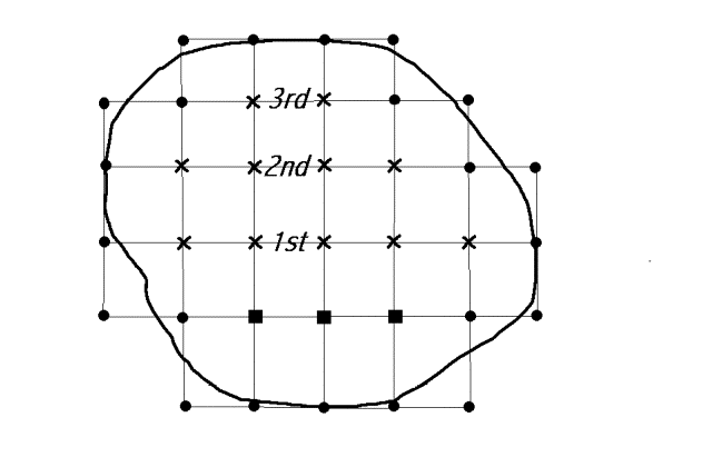
Figure 3: The marching
scheme for an arbitrary shape. The dots designate the boundary nodals and
interpolated/extrapolated boundary nodals, whereas the squares designate the
unknown nodals that are needed for the march towards 1st, 2nd,
3rd and the top boundary nodals. In this particular geometry only 3
unknown nodals are sufficient.

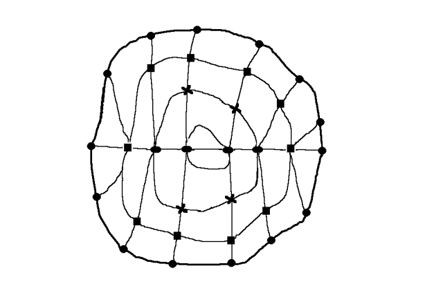
Figure 4: The nodals for an arbitrary geometry and irregular
shaped grid elements. For the elements the LPDE scheme of Fig. 1 is to be used
with interpolation/extrapolation weights. In actuality , though not well conveded
in the figure, the lines connecting the
nodes are well defined curves. The strategey of march is here from the unknown
5 squares at the bottom and the other 5 squares at the top the march is towards
the center line (with ovals). There and at the opposite walls the match will
give the values of the unknown nodals.